01
End-state method
Uses snapshots from bound and unbound end states rather than an explicit physical binding pathway.

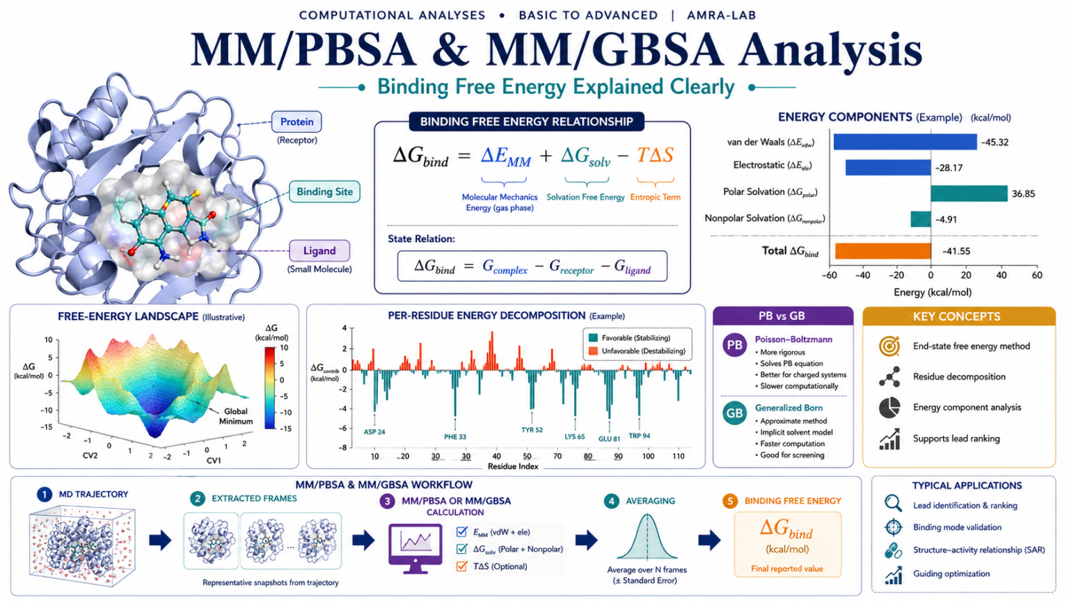
How end-state binding-energy estimation works, what each energetic term means, how PB and GB differ, how to interpret negative or positive values, and when these methods are useful or misleading.
Uses snapshots from bound and unbound end states rather than an explicit physical binding pathway.
Combines molecular-mechanics, polar solvation, nonpolar solvation, and optional entropy terms.
Often most useful for ranking related systems analyzed with one consistent protocol.
They are post-processing, end-state approaches used to estimate molecular association energetics from ensembles of structures, usually taken from MD simulations.
MM means molecular mechanics. PBSA means Poisson–Boltzmann surface area. GBSA means Generalized Born surface area. Both estimate a binding-energy change by comparing the complex with its receptor and ligand components.
They are widely used for protein–ligand, protein–protein, protein–nucleic acid, and other noncovalent complexes. They are computationally cheaper than many rigorous alchemical free-energy methods, but they involve important approximations.
Lennard–Jones interactions reflecting steric packing and dispersion. Often favorable when interfaces pack well.
Coulombic interactions between atomic charges. Can be strongly favorable before solvation penalties are included.
PB or GB estimates the cost or benefit of moving charged/polar groups between solvent exposure states.
Usually estimated from solvent-accessible surface area and represents cavity formation and nonpolar solvent effects.
Bond, angle, and torsional terms. In a single-trajectory protocol these often cancel substantially.
Accounts for loss or gain of configurational freedom. Frequently omitted because it is noisy and expensive.
ΔGbind ≈ ΔEvdW + ΔEele + ΔGpolar + ΔGnonpolar − TΔS
| Feature | MM/PBSA | MM/GBSA | Practical meaning |
|---|---|---|---|
| Polar solvent model | Numerical Poisson–Boltzmann equation | Generalized Born approximation | PB is often slower; GB is usually faster. |
| Speed | Moderate to expensive | Faster | GB can be convenient for larger frame sets. |
| Parameters | Grid, ionic strength, dielectric, radii | GB model, radii, dielectric, salt treatment | Settings strongly affect results. |
| Robustness | Can better represent complex electrostatic boundaries | Can be efficient but model-dependent | Neither is universally superior. |
| Best use | Consistent comparative studies with validated PB setup | Rapid comparative screening with validated GB setup | Benchmark against known systems whenever possible. |
Use equilibrated production frames, correct periodic-boundary artifacts, and verify the complex visually.
Create correct index groups and ensure all required cofactors, ions, or nucleic-acid chains are assigned consistently.
Choose single-, separate-, or multi-trajectory calculation according to the scientific question.
Use frames across a justified equilibrated interval. Avoid choosing only visually favorable snapshots.
Evaluate molecular-mechanics energy, PB or GB polar solvation, nonpolar solvation, and optional entropy.
Inspect cumulative averages, block averages, standard errors, autocorrelation, replicas, and sensitivity to settings.
Adjust energetic components and see how compensation between favorable interactions, desolvation, and entropy changes the apparent binding estimate.
Values are illustrative and intended for teaching.
More negative values are commonly interpreted as more favorable under the same protocol, but uncertainty and protocol sensitivity must be considered.
Binding often restricts translation, rotation, side-chain motion, loop motion, and ligand conformational freedom. This can create an unfavorable entropy penalty.
Common approaches include normal-mode analysis, quasi-harmonic analysis, and interaction-entropy-type approximations. Each has assumptions and noise.
Decomposition estimates how residues or residue pairs contribute to the calculated interaction-energy model. It can highlight candidate hotspot residues, favorable hydrophobic packing, electrostatic contributions, and unfavorable regions.
More negative contributions are shown with longer bars.
Complex, receptor, and ligand coordinates are extracted from the same complex trajectory. Internal bonded terms largely cancel and statistical noise is usually lower.
Limitation: It assumes receptor and ligand do not undergo major conformational reorganization on binding.
Complex, receptor, and ligand are simulated independently. This can account for conformational reorganization but usually has much larger uncertainty because large internal-energy differences no longer cancel.
Independent replicas help reveal sampling variability and reduce the risk of conclusions being driven by one trajectory.
Within an identical, validated protocol, a more negative calculated value is often interpreted as more favorable association.
However, differences should be larger than uncertainty and consistent across replicas, frame windows, and reasonable parameter choices.
A positive value suggests the included energetic terms do not favor association under that model. It may indicate weak binding, bad pose, poor sampling, incorrect protonation, topology problems, or strong desolvation/entropy penalties.
These are approximate end-state estimates. Absolute values may contain systematic offsets and depend strongly on the selected protocol.
Thousands of adjacent frames are not thousands of independent samples. Use block analysis or other correlation-aware uncertainty assessment.
Force fields, radii, dielectric constants, PB/GB models, salt, frame ranges, and entropy treatment can all shift results.
Cherry-picking produces biased estimates. Define the production interval before seeing the energy result.
Inspect trajectories, distances, contacts, RMSD, and pocket occupancy before interpreting averaged energies.
Decomposition is model-dependent and not a unique physical partition. Use it for hypotheses, not absolute claims.
gmx_MMPBSA is based on AMBER's MMPBSA.py and performs end-state calculations using GROMACS-generated files. A typical protein–ligand calculation requires a run input/structure, trajectory, topology, index groups, and an MM/PB(GB)SA input file.
&general
  startframe=1,
  endframe=1000,
  interval=10,
  verbose=1,
/
&gb
  igb=5,
  saltcon=0.150,
/
&pb
  istrng=0.150,
/
&decomp
  idecomp=1,
  print_res="within 6"
/
Use only the calculation namelists you need. Validate GB/PB settings for your system and current software version.
gmx_MMPBSA -O \
  -i mmpbsa.in \
  -cs complex.tpr \
  -ct md_center.xtc \
  -ci index.ndx \
  -cg 1 13 \
  -cp topol.top \
  -o FINAL_RESULTS_MMPBSA.dat \
  -eo FINAL_RESULTS_MMPBSA.csv
-cg takes the receptor and ligand group numbers. Confirm group IDs from your own index file rather than copying these example numbers.
Only as a comparative interpretation within the same validated protocol, and only when the difference exceeds uncertainty.
Not as interchangeable absolute values. Compare trends separately and validate each model.
There is no universal number. Frame spacing, correlation time, system flexibility, replicas, and convergence matter more than a fixed count.
Standard workflows usually use implicit solvent, but selected tightly bound waters may be retained in specialized protocols if treated consistently and justified.
They may perform poorly when ligands differ greatly in charge, size, binding mode, protonation, or conformational reorganization. Validation is essential.
It can suggest candidates, but combine it with structural persistence, alanine scanning, experimental knowledge, and replicas.
MM/PBSA and MM/GBSA are approximate, ensemble-based end-state methods. They are strongest as carefully validated comparative tools, not as automatic sources of exact absolute binding affinity.
Educational content for AMRA-LAB Computational Analyses · MM/PBSA & MM/GBSA module